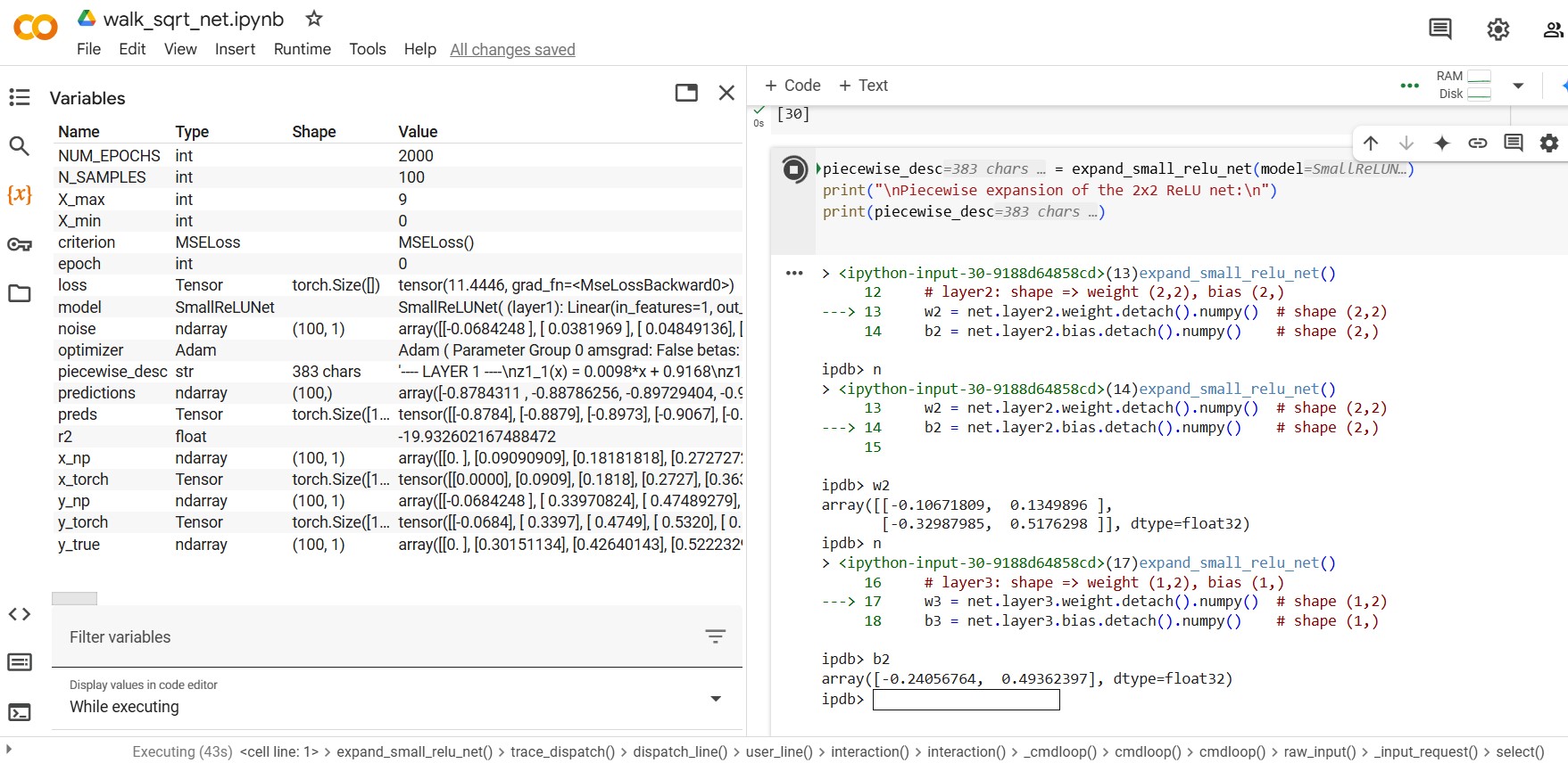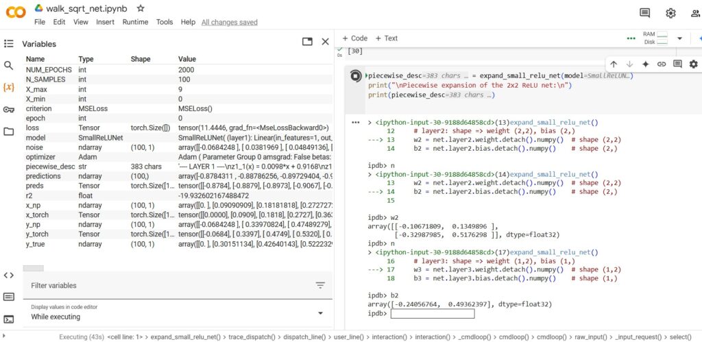
[walk_sqrt_net.py running as Python notebook in Google Colab, using set_trace() inline debugger to view neural-network weights/biases]
As part of applying software reverse engineering to AI, I’ve been working with OpenAI’s ChatGPT and Anthropic’s Claude.ai on writing Python code to inspect
neural networks. This has included an “InterpretableNeuralNet” that I’ll be describing in detail soon. From working on one part of the InterpretableNeuralNet, related to something called “surrogate polynomial coefficients,” ChatGPT and I backed into something much simpler that I’ll be discussing here: small programs that “walk” a neural net, i.e., follow an input value x through each element of the net to output value y, multiplying and adding the net’s weights and biases along the way (and adjusting for what ChatGPT below calls “kinks” in the net represented by threshold functions).
Note that large language models (LLMs) like ChatGPT and Claude are themselves neural networks, in many ways like the tiny toy nets that ChatGPT creates in the Python code below, though of course much larger. In the discussion below, ChatGPT compares and contrasts LLMs like itself with these toy nets. And while we start off discussing purely numeric neural nets, which are easier to understand, we wind up at ones that (like ChatGPT itself) have text input/output. Even if the reader isn’t interested in how AI can approximate the square root of x (y=sqrt(x), or x -> sqrt(x)) — without being given any knowledge of square roots (or even of techniques like regression) other than a sample of (x,y) data — please bear with ChatGPT and me as we’ll end up (in Part 2 of this article) creating and inspecting a small neural network that turns a word like “hello” into the predicted next word, “world” (“hello” -> “world”).
As context, those surrogate polynomial coefficients I mentioned above let one see what formula has been learned by a neural network that is trying to model some function like y=f(x). It’s a powerful method, one of five implemented by the InterpretableNeuralNet (which was originally created by Claude, and then modified by ChatGPT). However, I was disappointed to learn what ought to have been obvious to me, which is that this information comes from the neural network’s behavior: the surrogate polynomial coefficients method basically takes the input X values, and the net’s predicted Y values, and determines what function turns X into Y. It interprets the net basically by doing regression on input_X and predicted_Y. That’s very useful, and we’ll cover it soon as part of a larger discussion of the InterpretableNeuralNet, but the important thing here is that it comes from the net’s input/output behavior — it does not come from the net itself, i.e. from its weights, biases, and threshold functions.
I pushed ChatGPT on this: why can’t we inspect the net itself, taking an input x value, multiplying it by weights, adding biases, doing, mumble, something with threshold functions, and showing how an x gets turned into a predicted y? After all, this is what the net itself is doing, after training, when someone is using it to make a prediction, right?
At the same time, I had previously been under a mis-impression that while a neural network can often model the underlying function from which input (x,y) data was produced, no such network could tell us anything explicit about what formula it had learned (in the way that non-neural-net top-down regression can tell us the formula, e.g. given a trendline Excel has graphed for your data, it will also happily provide you the formula represented by that trendline and the error (R^2) by which that formula is “off” from your data). Inability of a neural net to tell us what function it is emulating — at the same time that the net itself has learned that function, and uses it in making predictions — is a serious problem, solutions or fixes for which come under names such as “interpretable AI” and “explainable AI“. But my belief in such nets’ total black-box opacity — absent some external reverse engineering based solely on its input/output without any inspection of its internals — was off the mark. ChatGPT here shows me that, if the neural net is small enough, we can see what de facto function it is implementing; it also shows that we can use such small-scale examples as background to understand large real-world LLMs.
Here’s much of the discussion we had, and the code “we” (i.e., ChatGPT) came up with. (ChatGPT below sometimes politely refers to “your code”, suggesting it’s discussing something I wrote, when it should know full well it wrote 99% of it, though under my direction.)
Why is this article so long? I could have just provided a summary of the discussion, together with the Python code and sample output, but including large portions of the discussion helps show the flavor or texture of conversing with AI chatbots, and of using AI to learn about AI. The style of conversing with ChatGPT is wordy, and probably not a model to be emulated in prompt engineering (especially given limits on window size and usage pricing), but it gets pedagogically-useful results.
(“Using AI to learn about AI”: I’ve put some cautions about this elsewhere in these articles, but it’s worth noting right here up front: LLMs such as ChatGPT or Claude do not have some privileged insight into their own operation. The incredibly useful things they can tell us about their own operation generally stems, not from “personal experience” or introspective knowledge of their own implementation, but from their vast reading of public research papers, articles, books, and source code — which in turn will sometimes reflect the LLM vendor’s documentation or open-source code, but which does not be confused with any self-knowledge. An LLM can help us understand LLMs in much the same way they could help us understand badminton or the political situation in Quebec, not in the way the developer of a program could try to help us understand that program. Nor, for that matter, in the way the program itself, by being open to reverse engineering, could help us understand the programming. There is a lot about reverse engineering AI here, but that’s distinct from “using AI to learn about AI” as the phrase was meant above.)
It’s worth seeing how carefully and patiently ChatGPT can work with me when I’m being deliberately dense, or truly dense, or when I explicitly tell it that I feel like my understanding is vague or confused. Sometimes (especially with Claude) I have to tell it, in effect, “hey, don’t humor me or give me soft soap with your ‘Oh you’re so absolutely correct, what an astute observation’ flattery; I want you to tell me where I’m off or confused.” That at least is a useful technique in prompting AI chatbots. One might ask whether chatbots organically learn sycophancy : does it comes naturally with next-word prediction (given texts it has trained on), and/or have they’ been deliberately tweaked to keep the interactions mildly addictive?
My prompts, and scattered commentary, in italics.
ChatGPT creates an initial tiny neural net, without hidden layers
[I’ve realized that my very first question to ChatGPT below, about whether something immediately useful “could be dug out of the net” in some case — even though it turns out to be accurate in a limited case — suggests a confusion about what a neural net consists of, and about what its weights are. A neural network’s “weights” are just that: weights. A node’s weight is a multiplier (positive or negative, small or large) that is applied to its input to help yield its output. A weight will only ever equal a readable coefficient in the simplest linear case. Furthermore, even in that limited case, a node’s weight reflects the function that the net has learned, not the net’s input data. The misimpression that an LLM “contains” something immediately readable, such as its own training data, is likely to appear in LLM copyright cases.]
AS: … I sort of vaguely thought that maybe a network can give us more of a formula when it finds a linear relationship between x and y, like “y=2.3x + 1.4” or something like that. Did I just make that up, or did I see something indicating that 2.3 and 1.4 could be dug out of the net in such a case? Or is that just another form of what’s happening here with surrogate polynomial coefficients?
ChatGPT o1:
Does a network ever give us a direct “formula”?
- If your network is purely linear (e.g., no hidden layers, just
y = w*x + b), you can indeed extract w and b directly from the model’s weights and say: “Here’s the exact formula.”
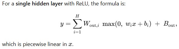
- In a multi-layer network with non-linear activations (ReLU, Tanh, etc.), the learned function is a piecewise polynomial or more complex shape. There’s no single closed-form expression that’s easy to read off just by looking at the weights. Instead, we use surrogates—like this polynomial fit—to approximate what the network does in a given input domain….
AS: Can you write a python script to illustrate this? Create a purely-linear network, provide some way to try out different w and b values, generate some (x,y) pairs, train the net, test e.g. with R^2 if it seems to have learned some meaningful relationship, and then walk the model’s weights to determine what w and b values are represented by the net?
ChatGPT o1:
[Thought for 5 seconds]
Below is a self-contained Python script illustrating how to train a purely linear PyTorch model y=w⋅x+b on synthetic data, and then extract the learned w and b directly from the model’s weights. We also compute R^2 to see how well it fits.
[AS: Yes, the o1 model thought all of 5 seconds to produce an initial 89-line script, linear_mode.py, that creates some (x,y) data based on the y=2.3x+1.4 example I gave in my earlier prompt to ChatGPT, uses that data (NOT the formula) to train the neural net so that, given a new x, it can try to predict the corresponding y, and then sees what formula the resulting net has implicitly learned in order to generate its predictions. Note that the Python code does not tell the net this formula. Nor would the net normally tell us what it has learned; normally a neural net simply behaves according to whatever formula it has learned from training, but won’t tell us what that formula is. Hence this exercise in reverse engineering neural nets, which in turn is related to Interpretable AI and Explainable AI (xAI).]
[AS: Below are ChatGPT’s commented enumerated sections in 89-line linear_mode.py :
# 1) Create synthetic data from y = w*x + b plus some noise
# 2) Define a purely linear model: one weight + one bias
# 3) Set up a loss function (MSE) + optimizer
# 4) Train the model
# 5) Evaluate R^2 on the training data
# 6) Extract learned W, B]
Explanation
- Data Generation
We pick a “true” slope TRUE_W=2.3 and intercept TRUE_B=1.4. We generate x from −5 to 5 and compute y=2.3x+1.4+noise. [AS: note that ChatGPT deliberately adds in some random noise, and that I hadn’t think to ask for this — benefits of noise are discussed below. For now, just note that these AI chatbots may go ahead and implement things (here, an excellent idea) you didn’t even think to ask them for.]
- Model Definition
A purely linear PyTorch model can be just nn.Linear(1, 1), i.e. one input dimension, one output dimension, no hidden layers. Internally, that’s exactly y=w⋅x+b .
- Training
- We define MSE loss (
nn.MSELoss) and use SGD optimizer. [AS: see MSELoss; SGD is explained in Part 2]
- We run for 5000 epochs, which is typically enough to converge on a small dataset.
- Extracting Weights
- In PyTorch,
model.linear.weight is a tensor of shape (1,1).
model.linear.bias is a tensor of shape (1,).- We use
.item() to get them as float scalars.
- Result
After training, we print the learned w and b. They should be close to the “true” values of 2.3 and 1.4, assuming the network converges well.
- We also compute R2, which should be near 1.0 for this simple linear problem with moderate noise.
Key takeaway: Because there are no hidden layers or non-linear activations, this is the entire formula. You can read off the final slope (weight.item()) and intercept (bias.item()) directly from the model.
AS: [Below, showing ChatGPT output from the Python code it wrote for me, and that I’ve run locally on a Windows laptop]
C:\work\ml>python linear_model.py
Epoch 0, Loss = 40.8855
Epoch 1000, Loss = 0.2433
Epoch 2000, Loss = 0.2433
Epoch 3000, Loss = 0.2433
Epoch 4000, Loss = 0.2433
Final R^2 on training data: 0.9945
Learned W = 2.2748
Learned B = 1.3756
True W = 2.3000
True B = 1.4000
I changed slightly. It seems to settle on correct w very quickly, b takes longer. Why would that be?:
C:\work\ml>python linear_model.py
Epoch 0, Loss = 39.6130, w=0.5190784931182861, b=0.7213650941848755
Epoch 100, Loss = 0.2480, w=2.295926570892334, b=1.2631158828735352
Epoch 200, Loss = 0.2410, w=2.295926570892334, b=1.3349626064300537
Epoch 300, Loss = 0.2409, w=2.295926570892334, b=1.3444910049438477
Epoch 400, Loss = 0.2409, w=2.295926570892334, b=1.3457547426223755
Epoch 500, Loss = 0.2409, w=2.295926570892334, b=1.3459221124649048
…
Epoch 900, Loss = 0.2409, w=2.295926570892334, b=1.3459447622299194
Final R^2 on training data: 0.9947
Learned W = 2.2959
Learned B = 1.3459
True W = 2.3000
True B = 1.4000
Also, it looks like the net is being initialized with random values, but I don’t see that in the code? [AS: I wanted to make sure it had random init, rather than the net being helpfully goosed to learn sqrt.]
ChatGPT:
Why Does w Converge Faster Than b?
It’s not uncommon to see the slope (w) “lock in” fairly quickly while the intercept (b) continues to adjust. A few possible reasons:
- Data Scale & Gradient Magnitude
- If your input x has a certain range (say, [−5,5], the partial derivative with respect to w might be larger on average than the partial derivative with respect to b.
- Larger gradient magnitudes can lead to faster parameter updates if you’re using a single learning rate (e.g., 0.01) for all parameters.
- Noise and Intercept Adjustments
- Even after w is nearly correct, the bias might still be “fine-tuning” itself to offset random noise in the training data.
- Because the cost surface with respect to b can be flatter (especially if the range of x is large and the model is close to correct), those updates might appear to move slowly. [AS: it would have been good to ask ChatGPT to explain “cost surface with respect to be can be flatter,” and even “partial derivative with respect to w,” even if I half understand what those mean, because AI chatbots in this context can be quite good at helping turn vague understanding into something specific.]
- Stochastic Gradient Descent Behavior
- If you used true SGD with mini-batches (in a larger dataset scenario), random sampling could affect how quickly b converges. (In your script you’re using the entire dataset each epoch, so this is less of a factor, but it still can play a role if you did random shuffling or mini-batches.)
[I later asked ChatGPT for simple explanations of SGD above, and other terms such as Kaiming/Xavier below. These explanations nicely relate the definition of the term to the very code we’re working with. I’ll put these in a separate page and link to them later in Part 2. For now, Wikipedia has reasonable explanations.]
In practice, if your final w and b are close enough to the true values — and your overall loss or R2 is good — it means the model is performing well. Whether b takes longer to settle is usually not a problem as long as it does converge.
Where Does the Random Initialization Come From?
PyTorch’s nn.Linear uses a default initialization strategy (often a form of Kaiming / Xavier uniform). By default, each time you create nn.Linear(in_features=1, out_features=1), PyTorch randomly initializes the weight and bias in a small range…
Because of that, every time you run your script, you’ll get a different random starting point unless you explicitly set a seed… [ChatGPT shows using np.random.seed(0) or torch.manual.seed(0)]. Doing that will make the initialization (and the subsequent training randomness) reproducible. Otherwise, PyTorch picks a different random seed each time you run the code, leading to slightly different initial w and b values—and sometimes a slightly different final solution if the dataset is small or noisy.
In summary
- Different runs yield different initial (w,b) because
nn.Linear has a built-in random initialization.
- Faster slope (w) convergence vs. slower intercept (b) convergence often happens due to differing gradient magnitudes and how the optimizer steps are applied.
- This is normal behavior, especially if the final fit quality (
R^2 ≈ 0.99+) meets your needs.
Walking a toy neural net with hidden layers
AS: I don’t think I appreciated that your “purely linear” meant not only that the (x,y) training data has a linear relationship, but also that there were no hidden layers, I realize this sounds very contrived, but for pedagogical purposes, would it be possible to have a hidden layer with some neurons whose weights/biases could be “walked” to arrive at the formula? By “walk”, I mean something like taking an input x, multiplying by first weight encountered, adding first bias, moving to next weight, etc., and eventually yielding y.
[Below, I’ve sometimes included ChatGPT’s “chain of thought” (CoT) as shown in a right-hand panel. Its phrases like “I’m thinking through…”, and references to its own apparent “considering” are at least intriguing, though see comments elsewhere on this site re: accuracy or faithfulness of these CoT details.]
ChatGPT:
[Thought for 13 seconds:
Piecing together the formula
I’m thinking through the function for a single hidden layer MLP with ReLU activation, considering the piecewise nature of ReLU transformations and the subsequent summation of weighted outputs.
[AS: MLP is not My Little Pony but multilayer perceptron (the linked-to Wikipedia article has a nice timeline going back to McCulloch/Pitts in 1943 and Frank Rosenblatt in 1958-1962, though surprisingly doesn’t mention Minsky/Papert’s famous or infamous chilling critique from 1969, which is thought to have delayed widespread adoption of the neural-network (non symbolic) approach to AI by over a decade). ReLU(x), which is essentially the max of zero and x, is a “rectified linear” unit, and is discussed later.]
Navigating the network
Piecing together a Python script to extract weights from a single hidden layer MLP. This script will effectively ‘walk the net’ using a contrived example.
Crafting the script
I’m mapping out a Python script to build and display formulas for a single hidden layer MLP, including data generation and a function for piecewise ReLU expressions.]
Below is a contrived example that demonstrates:
[AS: below, I like ChatGPT’s “linear-ish”. I especially like its “plus noise for illustration” (note that I didn’t ask for this). While I should have asked it to explicitly state how adding some random noise helps illustrate points this code is trying to make, surely two reasons are (1) to underline that the net isn’t simply top-down learning some rote formula, but is instead going to reach its results “from the bottom up” based on the data; and (2) introducing some noise should help the net avoid “overfitting”, discussed below.]
- A tiny neural network with a single hidden layer (two neurons) and ReLU activation.
- Training it on some linear-ish data (you can pick any function—here we just do y=2.3x+1.4 plus noise for illustration).
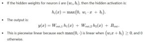
- “Walking” the network’s weights to see how an input x flows through each layer. Because of the ReLU, the final formula is piecewise linear — one piece for when each neuron’s pre-activation is ≥0, and another piece for when it’s < 0. [AS: the “piecewise” nature of neural nets is discussed below.]
Disclaimer: For bigger or deeper networks, this piecewise expansion becomes unwieldy. But for a single hidden layer with a small number of neurons, you can indeed write out the entire function by hand from the weights.
[AS: See linear_model_2.py ; ChatGPT’s commented enumerated sections from the 141-line script:
# 1) Synthetic data from a known linear relationship: y = 2.3x + 1.4
# 2) Define a net with one hidden layer, no activation
# 3) Train the model with MSE Loss + SGD
# 4) Evaluate with R^2
# 5) Show the model’s raw parameters
# 6) “Walk” the formula manually
# 7) Combine everything into an “effective” slope & intercept]
How It Works
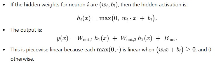
- SingleHiddenLayer:
layer1 is a linear map from R1→R2. That yields 2 neuron outputs.nn.ReLU() is applied element-wise, so each neuron is max(0,wix+bi).layer2 is a linear map from R2→R1, so we have an output weight for each hidden neuron plus one output bias.
- During Training:
- We use MSE loss and simple SGD.
- The net tries to approximate y=2.3x+1.4 with noise. Because it’s only 2 ReLU neurons, it can represent a piecewise linear function.
- Extracting the Formula:
4. Printed Output
Summary
- Yes, you can manually “walk” a network’s hidden weights to produce a piecewise formula.
- For deeper or larger networks, the expression quickly becomes more complex.
- But for small contrived examples, it’s perfectly feasible — and helpful for pedagogical illustration!
[AS: above, note especially ChatGPT’s references to a “piecewise” function and to “kinks” or “breakpoints” in the function. The point is that once we add threshold functions such as ReLU to the network, we can no longer simply “walk” it by multiplying preceding value by the node/neuron’s weight, then adding in the bias. What would otherwise be a simple “y=bias; for each i, y += (weights[i] * input[i])” has to break at each ReLu() to possibly be zeroed. Though also note, as discussed below, ReLU is simply “((x) > 0.0 ? (x) : 0.0)”.]
AS: Thank you for humoring me. This is actually very useful.
[AS: below I just show ChatGPT, without any explanation or question, output from the code it had written, which I had dutifully run on my laptop, and ChatGPT walks me through what the output is telling us.
[As you can perhaps tell, it’s a little too easy to get into a rhythm where ChatGPT or Claude create or modify source code for you, you blithely run the code locally with hardly a glance at what the code says, report the results back to the chatbot, and a few seconds later it tells you what the problem is, and gives you a revised file to run. It’s generally better to just get snippets representing the change (even though getting back an entirely new source-code file is easier), because you at least feel you have some agency when you’re copy/pasting in a discrete modification. I have seen myself becoming very routinized in these coding sessions with ChatGPT and Claude.
[At any rate, the reader can see below that, whereas the true formula for the input (x,y) data is y=2.3x+1.4, plus some noise, the neural net from the (x,y) data alone, without being told the formula, after 2000 training “epochs,” learned that y = x * 2.3041 (slope) + 1.3241 (intercept). The reader may ask, can’t we get it to exactly y=2.3x+1.4 if we just let its training run longer? Well, for one, there was that random noise added in to the (x,y) input data, so for all we know y=2.3041*x + 1.3241 could more closely match the input data.
[But more important, one generally doesn’t want a neural net to precisely represent the input (x,y) data, because while that might even lead to accurate interpolation of values it hasn’t seen before, it often leads to “overfitting,” with humorously-wrong extrapolations on input values outside the range of its input data. This was presumably a reason ChatGPT’s added in some randomness: we want these nets to learn general rules that conform to the input training data, so that the net can predict new values it hasn’t seen before, outside the range of its training data; we don’t want them to over-generalize so that all they do is so closely match the training data without making useful new predictions. We want the net to learn, NOT to memorize. We don’t want to create some complicated lookup table.
[As a final point on noise, and as a general reverse-engineering point, note the difference between an as-designed function or structure (de jure) vs. an actual as-built function or structure (de facto), with the noise that was added in here perhaps standing in for everything that can happens between a project’s de jure plans on the one hand, and what gets built de facto, on the other hand. That difference will often be more substantial than the minor difference here of y=2.3041x+1.3241 vs. y=2.3x+1.4 .]
C:\work\ml>python linear_model_2.py
Epoch 0, Loss = 37.7567
Epoch 1000, Loss = 0.1824
Epoch 2000, Loss = 0.1824
R^2 on training data: 0.9960
Hidden layer weights:
[[ 1.4522533]
[-0.3203768]
[ 0.2639456]]
Hidden layer bias:
[ 0.97776866 -0.644724 -0.20064451]
Output layer weights:
[[ 1.436641 -0.3684002 0.3776308]]
Output layer bias:
[-0.242365]
Derived step-by-step formula:
z_0(x) = (1.4523)*x + (0.9778)
z_1(x) = (-0.3204)*x + (-0.6447)
z_2(x) = (0.2639)*x + (-0.2006)
y(x) = (1.4366) * z_0(x) + (-0.3684) * z_1(x) + (0.3776) * z_2(x) + (-0.2424)
Effective single-layer slope = 2.3041
Effective single-layer intercept = 1.3241
True W = 2.3000
True B = 1.4000
ChatGPT: It looks like you ended up with a one-hidden-layer network (3 hidden neurons in this case), and then manually “walked” the final weights/biases to derive a piecewise-linear (or in your printout, purely linear if no activation is used) function that relates x to y. You also combined them at the end to get an “effective” single-layer slope and intercept. That final line:
Effective single-layer slope = 2.3041
Effective single-layer intercept = 1.3241
shows how the net’s entire set of transformations (layer by layer) can be collapsed into a single linear equation. It’s very close to the true slope/intercept (2.3, 1.4)
Below is a quick recap of why that works and what each part means:
1. Hidden Layer Weights & Biases
From your snippet:
Hidden layer weights:
[[ 1.4522533]
[-0.3203768]
[ 0.2639456]]
- This indicates each hidden neuron hi (for i=0,1,2) has:
zi(w) = wi⋅x+bi
where wi and bi come from the lines above.
In your code snippet, it looks like you might not be applying a ReLU or any nonlinearity in that hidden layer—otherwise you’d see max(0, z_i).
- If that hidden layer had a ReLU, you’d see something like:
hi(x)=max(0, zi(x))
But since your print-out shows direct usage of z0(x), z1(x), etc., it seems you might have a purely linear hidden layer (i.e., no activation). That effectively just folds into a single linear transform overall—like a matrix multiply.
2. Output Layer Weights & Bias
This means your output y is:
y(x) = 1.4366 ⋅ z0(x) − 0.3684 ⋅ z1(x) + 0.3776 ⋅ z2(x) − 0.2424
Hence your final line:
3. Why This Can Fold into a Single Linear Equation
A) No Nonlinearity?
If the hidden layer is truly a linear layer (with no ReLU, Tanh, Sigmoid, etc.), then two consecutive linear layers are mathematically equivalent to one linear layer. In other words:
Linear2(Linear1(x))=A(Bx+b1)+b2=(AB)x+(Ab1+b2)
which is just a single matrix multiplication plus a single bias vector.
Hence your “Effective single-layer slope” ≈2.3041 and “Effective single-layer intercept” ≈1.3241
B) If There Were a Nonlinearity
If the hidden layer had a ReLU or Tanh, you’d get a piecewise-linear or nonlinear expression that does not collapse so simply into a single linear equation. You’d see multiple pieces or segments.
4. Interpretation
- Good Fit: The final numbers match the true slope (2.3) and intercept (1.4) fairly closely—hence a high R².
- Why Intercept Slightly Off?: Just typical minor differences due to noise, random initialization, and finite training steps.
- Pedagogical Value: This exercise shows how you can interpret a multi-layer net’s function if there’s no nonlinearity in the hidden layer. It’s basically the same as a single linear layer. Or, if there is a nonlinearity, you can still expand out all the weights and see the piecewise or polynomial structure—but that can get complicated fast if you have more layers or bigger hidden sizes.
Conclusion:
- You’ve effectively verified that if you don’t use any nonlinear activation in the hidden layer, a “2-layer net” is just a single linear function (it can be collapsed).
- By printing out the intermediate “z_i(x)” equations, you see the chain of matrix multiplies and biases. Summing them all up yields a single slope and intercept that approximates your original linear function y=2.3x+1.4 .
How’s this apply to larger neural networks?
AS: Question about the last thing you said above:
>>> By printing out the intermediate “z_i(x)” equations, you see the chain of matrix multiplies and biases. Summing them all up yields a single slope and intercept that approximates your original linear function y=2.3x + 1.4
Presumably this ability to walk a neural network and sum up the weights and biases is also true of much larger, more complex networks. I mean, isn’t that exactly what the net itself is doing to turn new x inputs into y outputs? Yes, threshold functions (which may be nonlinear) are getting applied in there, but there is basically a set of multiplications and additions going on. Except in the unlikely chance I have this 100% correct, please tell me where I’m wrong, or what I’m missing.
[AS: below, see how ChatGPT followed through on my “please tell me where I’m wrong, or what I’m missing” request. And note the major points it is making about the nature of neural nets as “piecewise” functions with “regions” (even the huge ones like ChatGPT are computing a function, albeit typically with “regions”/”pieces”/”kinks”). Later, I push back a bit on whether the presence here of ReLU(), which is simply max(0,x), really undermines the net’s otherwise “closed form” expression.]
ChatGPT:
Thought for 14 seconds
You’re basically correct that for any neural network—no matter how big—you could, in principle, “walk” through every weight and bias to produce a literal mathematical expression for how an input x (or vector x) becomes an output y. After all, a network is just a chain of (linear transformations) + (nonlinear activations).
However, there are two big caveats:
- Nonlinear Activations Create Piecewise or More Complex Expressions
- A purely linear layer (no activation) collapses into a simple matrix multiplication plus a bias (i.e., one set of “slope” and “intercept” if you have a 1D input, or a single matrix if you have higher dimension).
- As soon as you add an activation like ReLU, Tanh, or Sigmoid, the network’s overall function becomes piecewise or otherwise more complicated. For instance, a ReLU-based network is piecewise linear, with each ReLU introducing a “kink” that depends on the sign of its input.
- In a deep network with many neurons, you get a combinatorial explosion of regions—potentially billions of linear “pieces.” Each piece can be written down, but the formula can become astronomically large.
- Practical Intractability
- Even though the net is “just” matrix multiplies + additions + elementwise nonlinearity, expanding that out by hand (or symbolically) for large architectures quickly becomes impractical.
- For a single hidden layer with a few neurons, it’s instructive to see exactly how max(0,wx+b) transforms your input, and how those transformations sum up.
- For many layers or neurons, you’d end up with an enormous piecewise definition or nested expressions that aren’t human-friendly.
Bottom Line
- Yes, from a purely mathematical standpoint, every neural network is a function you can “expand.”
- Yes, the net itself is computing that function—just in a structured way (layer by layer). [AS: later we’ll get into how a hierarchy of layers can shape or filter lower-level input into higher-level constructs (or at least what might be viewed that way); see “cat ears” in forthcoming page on “features” and the “InterpretableNeuralNet”.]
- But, once you add typical nonlinearities (like ReLU), each layer’s output depends on conditions like wi⋅x+bi≥0. In a large net, you get an exponential number of regions, making the full expression unwieldy to write down or interpret.
So you’re 100% correct that there’s nothing stopping you from deriving the network’s piecewise or nonlinear formula step by step. It’s just that, for bigger architectures, such a formula is too large to be practical as a neat “closed form” expression—whereas for a small net (a single hidden layer with a couple neurons), you can see exactly how it works.
A walkable neural net that models the square root function
AS: I wonder if the presence of ReLU, Tanh, or Sigmoid really complicate things that much, given that ReLu(x) for example is simply max(0,x); sigmoid(x) is (less simply) 1/(1+exp(-x)); tanh(x) is, okay, more complicated, but a bunch of exp() calls.
So isn’t it largely the explosion with a larger network that makes this impractical?
Could you try this with a much smaller version of the net [“InterpretableNeuralNet” computing square root, log, rand, etc. to be discussed elsewhere] that you’ve been working on for me? That’s all ReLu. You could cut back the 3×256 layers to 2×64 if that would help. So long as it could do a moderately plausible job of modeling y=sqrt(x) for example.
ChatGPT:
[Thought for a second] [AS: yes, it was like one second]
Yes, the main issue in “expanding” a neural network’s computation into a closed-form symbolic expression is combinatorial growth of the terms/regions when the network has many neurons/layers with nonlinear activations. Each ReLU introduces a piecewise condition (“if w⋅x+b≥0 then ………, else ………”), and in a multi-layer net with many neurons, the number of possible “pieces” can explode.
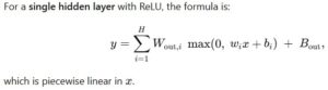
However, for a small ReLU network—say 1 or 2 hidden layers with a small number of neurons—you can write out a piecewise-linear function explicitly, and it’s still instructive to see how the hidden units combine in a final formula.
Below is a self-contained example:
- We define a small ReLU network with two hidden layers.
- We train it on y=sqrt(x) (with some noise). [AS: as always in this ChatGPT session, this means we train it on data that was generated using sqrt(x); we do not tell the network anything about sqrt(x).]
- We expand out (manually) all the ReLU-based piecewise expressions. Because we keep the net small (2 layers of 2 neurons each), it’s still somewhat readable.
Note: This is still somewhat contrived—any bigger and you’ll get a lot of piecewise conditions. But it demonstrates how you could do it.
Full Example: 2-Layer ReLU Net, 2 Neurons Each, Modeling sqrt(x)
[See walk_sqrt_net.py; ChatGPT’s enumerated comments in the 149-line script:
# 1) Synthetic data: y = sqrt(x) on [0..9], plus some noise
# 2) A small ReLU network with two hidden layers, each has 2 neurons
# 3) Train the model on sqrt(x) data
# 4) Evaluate performance
# 5) Expand the network manually into a piecewise function
# 5a) Extract parameters
# 5b) “Stringify” each part
Also see Python notebook (walk_sqrt_net.ipynb) at Google Colab, as shown in earlier screenshot; in Colab, press {x} to see the variable window.] [[TODO: ipdb.set_trace() debugger calls in .pynb may be broken in shared version]]
The code defining the neural network, and the training loop, are shown below; also see neural-network diagram towards the end of this page:
###############################################################################
# 2) A small ReLU network with two hidden layers, each has 2 neurons
###############################################################################
class SmallReLUNet(nn.Module):
def __init__(self):
super(SmallReLUNet, self).__init__()
self.layer1 = nn.Linear(1, 2) # from x to 2 hidden units
self.layer2 = nn.Linear(2, 2) # from 2 hidden units to 2 hidden units
self.layer3 = nn.Linear(2, 1) # from 2 hidden units to output
self.relu = nn.ReLU()

def forward(self, x):
# 1) hidden1
z1 = self.layer1(x)
a1 = self.relu(z1)
# 2) hidden2
z2 = self.layer2(a1)
a2 = self.relu(z2)
# 3) output
out = self.layer3(a2)
return out

model = SmallReLUNet()
criterion = nn.MSELoss()
optimizer = optim.Adam(model.parameters(), lr=0.01)

NUM_EPOCHS = 2000
for epoch in range(NUM_EPOCHS):
optimizer.zero_grad()
preds = model(x_torch)
loss = criterion(preds, y_torch)
loss.backward()
optimizer.step()
What You’ll See
- Training
- The net tries to approximate sqrt(x) on
[0..9]. With only 4 hidden neurons total (2 in each layer) and ReLU activation, it might do an okay job, but not perfect.
- You should get a final
R^2 anywhere from ~0.95 to ~0.99, depending on random initialization, training steps, etc.
- Piecewise Formula
You’ll see something like:
Each max(0, ...) defines a piecewise condition. For instance, if z1_2(x) < 0, then a1_2(x) is 0 for that range of x. That changes the slope for that region.
- Why It’s Still “Small”
- We only have 2 neurons in each layer, so we have a total of 2 “ReLU gates” in the first hidden layer, and then 2 “ReLU gates” in the second hidden layer. That leads to up to 2×2=4 potential “kink” conditions.
- This is still fairly human-comprehensible (though not trivial).
- Scaling Up
- If you had 64 neurons per layer, you’d get 64 ReLUs in the first layer, 64 in the second, leading to a far bigger piecewise expansion. It quickly becomes unwieldy to read.
Why the Nonlinearities Are a Big Deal
- If there were no ReLUs, then consecutive linear layers collapse into one linear transformation (as we saw). That’s easy.
- If you do have ReLUs, each one is
max(0, …). Over multiple layers, each input dimension to each subsequent layer depends on whether the preceding ReLUs were “on” or “off.” This yields a piecewise linear function with exponentially many regions in the worst case.
[AS: ChatGPT’s “a Big Deal” is likely in response to my seeming to underplay it when trying to cajole ChatGPT a bit into generating this code. Clearly it is a big deal as it relates to what it amusingly calls “kink” conditions, and to ChatGPT’s point above: “Each max(0, …) defines a piecewise condition. For instance, if z1_2(x) < 0, then a1_2(x) is 0 for that range of x. That changes the slope for that region.”]
In your tiny 2-layer / 2-neuron example, that exponential blow-up is still small enough to illustrate. As soon as you scale to “2×64,” it’s mathematically the same principle, but enumerating 64 ReLUs in each layer is monstrous.
Summary
- Yes, any neural net is “just” a composition of linear transforms and simple non-linear functions like ReLU max(0,x) .
- You can absolutely expand that function into a piecewise or nest of expressions.
- But the complexity grows quickly. For a “2 layers × 2 neurons each” net, you can handle it. For “2 × 64,” you might not even want to see the final piecewise form.
- This example demonstrates the concept for a small ReLU net trained on sqrt(x). Once you see it in action, you get how quickly it becomes unwieldy at larger scales.
AS: Thank you for doing this for me. Very helpful! Output: [not sure why I’ve got in the habit of thanking it, and giving it verbal gold stars, since the UI provides a place to give a thumbs-up or thumbs-down which, unlike this polite tic of mine, might actually be useful.]
At my request, ChatGPT later gave me a graph of SmallReLUNet which Mermaid rendered, and which may be helpful while staring at the program’s output below:
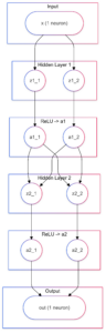
Running the program:
C:\work\ml>python walk_sqrt_net.py
Epoch 0 | Loss = 4.2715
Epoch 500 | Loss = 0.0337
Epoch 1000 | Loss = 0.0337
Epoch 1500 | Loss = 0.0337
Final R^2 on training data: 0.9385
Piecewise expansion of the 2×2 ReLU net:
—- LAYER 1 —-
z1_1(x) = -0.7722*x + -0.2687
z1_2(x) = 0.5862*x + 0.2965
a1_1(x) = max(0, z1_1(x))
a1_2(x) = max(0, z1_2(x))
—- LAYER 2 —-
z2_1(x) = 0.0055*a1_1(x) + -0.0440*a1_2(x) + -0.5258
z2_2(x) = -0.6184*a1_1(x) + 0.9509*a1_2(x) + 0.3176
a2_1(x) = max(0, z2_1(x))
a2_2(x) = max(0, z2_2(x))
—- LAYER 3 (Output) —-
out(x) = 0.2311*a2_1(x) + 0.4904*a2_2(x) + 0.4774
[[TODO: given a specific example like x=5, go through the 3 layers, showing how input 5 becomes output ~ 2.236; use output from walk_sqrt_net_2.py, but need to walk a little slower through the following so see how, in the trained net, 5 becomes 2.2318
Enter x values to see step-by-step ReLU net output (type ‘q’ to quit).
Enter x (or ‘q’): 5
True sqrt(5.000) = 2.2361
Net prediction: 2.2318
Step-by-step values:
z1_1 = 2.9044, z1_2 = -0.9108
a1_1 = 2.9044, a1_2 = 0.0000
z2_1 = 0.3628, z2_2 = -1.6956
a2_1 = 0.3628, a2_2 = 0.0000
out = 2.2318
Enter x (or ‘q’): 8
True sqrt(8.000) = 2.8284
Net prediction: 2.8261
Step-by-step values:
z1_1 = 4.6308, z1_2 = -1.1413
a1_1 = 4.6308, a1_2 = 0.0000
z2_1 = -0.2034, z2_2 = -2.6673
a2_1 = 0.0000, a2_2 = 0.0000
out = 2.8261
But outside of training range [0..9], starts to fail badly:
Enter x (or ‘q’): 10
True sqrt(10.000) = 3.1623
Net prediction: 2.8261
Step-by-step values:
z1_1 = 5.7817, z1_2 = -1.2950
a1_1 = 5.7817, a1_2 = 0.0000
z2_1 = -0.5808, z2_2 = -3.3152
a2_1 = 0.0000, a2_2 = 0.0000
out = 2.8261
See earlier discussion of overfitting, extrapolation vs. interpolation; discuss what it means to “learn sqrt” (maybe use Google Gemini’s way of explaining it?); also note log, rand, tan.]]
Interim conclusion for Part 1
This article has gone on too long for a single web page; much more will appear soon in a separate lengthy page with Part 2. Here’s key points from what we’ve discussed so far:
- Large language models (LLMs) such as ChatGPT, Claude, and Google Gemini, are, at bottom, neural networks.
- Even the largest neural net, like ChatGPT itself, after its has been trained with sample data, computes a function: y=f(x) .
- A neural net can approximate the effect of a function such as square root (and log, tan, etc.), without ever knowing that’s the function it is approximating, and based only on some sample (x,y) training data that was generated by the function.
- Neural networks are overly opaque (non-transparent) for many applications: while the net can amazingly compute all manner of things (including an appropriate next word in a sentence), they are currently much less good at telling us how/why they arrive at their y outputs, given x inputs.
- However, they are not totally opaque; neural networks can be reverse engineered.
- In addition to applying post-hoc analysis to neural networks, such as surrogate polynomial coefficients, in certain limited cases one can “walk” through the neural net to extract the formula a neural net has learned, directly from the net’s weights/biases.
- Any non-trivial neural net, once it uses nonlinear activation functions such as ReLU, will contain “kinks” or regions; each seem between regions is marked by an activation function.
- We don’t want a neural net to memorize its (x,y) training data; we want to net to learn the (x,y) relationship, which is very different; we don’t want the effect of a lookup table; instead, we want something that can predict y give input values x the net hasn’t seen before; we want neither “overfitting” nor “overfitting”; we want the net to learn both accuracy and generalization.
- We saw an extended example of interacting with an AI chatbot like ChatGPT to produce code and assess its output, when the user runs the code locally.
Topics discussed in Part 2 will include:
- Apply net-walking from small neural nets representing numeric data to those representing text
- Similarities and differences from LLMs
- Walking a tiny toy language model
- What text “embeddings” represent in the tiny language model, compared/contrasted with embeddings in LLMs
- Temperature, argmax/softmax, logits, sampling, and selecting the next token from a list of the most-probable next tokens
- Historical comparison of finding square root by guessing/iterating, with the neural net’s method of training/error-adjusting weights
- Other resources that examine neural networks at a low level
- The 768 “sweet spot”
- The separate roles of backpropagation vs. the optimizer
- Transformers and “attention” are NOT performing recurrence, though it can appear that way in a chat
- Transformers like ChatGPT are “just like” our tiny neural networks, except…
Other forthcoming topics on reverse engineering AI here at softwarelitigationconsulting.com will include:
- Do neural networks truly discover “features” implied or inherent in their input data, and how?
- InterpretableNeuralNet: Explainable AI (xAI) and neural network interpretability with activation capture, hooks, local linear approximation, sensitivity analysis, extracting surrogate coefficients, visualizing layer activations with heatmaps, showing the “top” activated neurons, etc.
- “Error correction is (almost) all you need” (cf. W. Ross Ashby: “The whole function of the brain is summed up in: error correction”)
- Neural networks, regression, and the Universal Approximation Theorem (UAT)
- AI chatbot “Chain of Thought” (CoT) and “introspection”
- Using sentence embeddings for patent claims to model geometric “spaces” into which patent claims (and corresponding technology) fit
- Developing an offline/local source-code examiner with open-source code-specific LLMs such as CodeLlama
- The relation of interpretable AI, explainable AI, and alignment on the one hand, with software reverse engineering on the other hand
- AI as both a tool in, and subject of, intellectual property litigation